< up >
2022-07-23

Saving Goats with Prolog

Preface

This post was originally posted in my old blog raphaelpour.de on 09.02.2018. Retrospectively this post is a pretty good insight of my artifical intelligence studies back then.

Spoiler: You might have guessed it already… you won’t see any real goat in here¹. This is about a planning problem and how we can solve it using Prolog. A planning ploblem could be for example a game or a more or less complex task. You know the starting and goal state and the rules to go from one state to another, but not if and how many states are between².

I will describe the problem, break it down to Prolog and solve it with an Iterative Depth Search (IDS).

Where are the Goats now?

Okay, first things first: There is only one goat. And this goat can only survive under specific circumstances.

Imagine you are a ferryman, going from one riverside to the other. Next to some rickety grandmas (which are taking the ferry almost every day to keep themselves busy) and a bunch of heavily interested tourists (not interested at all), you were commissioned to transport three things from riverside A to riverside B:

• goat
• cabbage
• wolf

Rules:

• only one thing at a time transportable
• goat eats Cabbage
• wolf eats Goat

How can the ferryman transport all three things from riverside A to B?

Breakdown of the Problem

Imagine playing a game which you never played before. The rules are clear but it might not be clear which strategy is key. The best strategy in the first place might be guessing or do things in a specific order to gain experience. To make the things more formal: When I have situation X, which action/move/… leads me to the goal situation?

Same thing in Prolog. We can implement the rules, but we need an algorithm which tries to find a solution. In order to find something, you have to search. While we have no heuristic (or in our game example: we have no experience) to rank all current possible actions by shortest distance to the goal, we need an uninformed search algorithm.

The most effective one is the Iterative Depth Search (IDS). It combines the positive aspects of the breadth-first- such as the depth-first search and is therefore optimal (finds always the shortest path).

The search algorithm can walk through a graph where the nodes are states and the edges are the action/move/… you have to do in order to go from one state to an other.

In our example, ervery state contains the location of four things: Goat, Cabbage, Wolf and Ferryman. Every thing can be either on riverside A or B. As a result every state is a combination of the location of all four things. The Rules are telling us which actions are allowed and which not.

Let’s imagine how a search graph would look alike (see graphic below). Each node is a state and each edge is an action.

But this graph has some faulty edges which are not following our rules. Guess which!

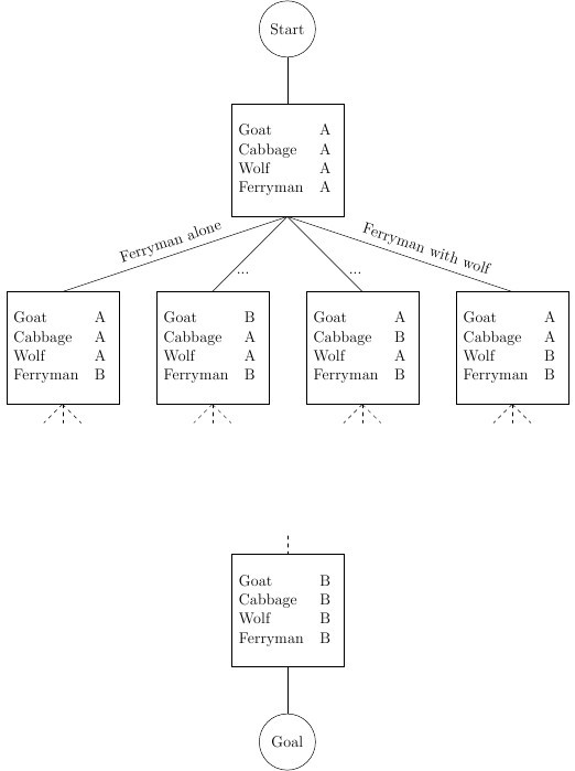
The following edges are wrong:

• edge 1: The ferryman is allowed to go alone, but either the goat is eating the cabbage or the wolf is eating the goat (or both).
• edge 3: The wolf is eating the goat.
• edge 4: The goat is eating the cabbage.

The Prolog Program

In order to make use of the search algorithm, we need to put every state into a List describing the location of each thing: [goat, cabbage, wolf, ferryman]. We start off by describing the start and goal state:

start([a,a,a,a]).
goal([b,b,b,b]).

Next we create a transition allowing the ferryman to go alone from riverside A to riverside B. This is accomplished by only allowing the ferryman variable to change the location, all other variables have to stay where they are.

transition0([G,C,W,a],[G,C,W,b]).

Let’s add all other transitions.

transition0([a,C,W,a],[b,C,W,b]). 
transition0([G,a,W,a],[G,b,W,b]).
transition0([G,C,a,a],[G,C,b,b]).

This Transition goes only in one direction. Let’s make it symmetric by adding a new transition predicate.

transition(X,Y) :- transition0(X,Y);transition0(Y,X).

The reason why I called the predicate transition and not rule is that the most rules are missing. We actually can move from A to B with only on thing at a time, but it is allowed to keep for example the wolf and the goat alone. We need to validate each state in order to tell if the transition is allowed or not. Let’s make a new predicate for the validation and add it later to our symmetric transition.

valid([F,_,_,F]).
valid([G,C,W,_]) :- G \== C, G \==W.

This predicate takes a single state and checks if:

• The Goat is with the ferryman -> Everything is okay because the wolf doesn’t harm the cabbage
• The Goat doesn’t share its location with either wolf or cabbage. We can exclude the ferryman here while we took care of him in the rule above

Now we can add the valid predicate to our transition.

transition(X,Y) :- (transition0(X,Y);transition0(Y,X)), valid(X),valid(Y).

Summary

• The transition0 Predicate describes which move is allowed from a to b.
• The valid Predicate checks if a single state is legal based on our rules.

The transition Predicate uses our transition0 in both directions in order to go from a to b and from b to a. This is possible while Prolog doesn’t have fixed Input and Output Variables.

The Search Algorithm (IDS)

As already mentioned, the Iterative Deepening Search Algorithm fits perfect for our needs. In order to understand how this search works, I will build it up step by step.

At first we need the depth-first-search on which the IDS is based on.

ds(Node, Goal) :-
    Node == Goal;
    transition(Node,Neighbour), ds(Neighbour, Goal).

The Depth-First search works with the Back-Tracking feature of Prolog. It goes into depth until either a Goal is reached or transition returns false. If the transition is false, it will go to the previous call of transition and will try all possible transition s until a goal has been reached or no transitions are left³.

This implementation doesn’t has a kind of a history in order to avoid infinite loops when the graph has a circle.

ds(Node, Goal, Path) :-
    Node == Goal;
    transition(Node,Neighbour), not(member(Neighbour,Path)),
    ds(Neighbour, Goal, [Neighbour|Path]).

Now out Search keeps track of the previous passed nodes and passes no node twice. Until now, our Search only returns a true or false whenever the goal can be reached or not. What’s with the path itself? Unfortunately, the path will be deleted when the search comes back from the recursion. This can be added by using an additional output variable. This will be filled with a reserved version of our path while the head of the path is the last move and the last element of the tail our start node.

ds(Node, Goal, Path, ReturnPath) :-
    Node == Goal, reverse(Path, ReturnPath);
    transition(Node,Neighbour), not(member(Neighbour,Path)),
    ds(Neighbour, Goal, [Neighbour|Path]).

Now we have and uninformed depth-first-search but the i is still missing. Let’s add a loop ids_loop that increases the depth until the goal has been reached. The loop is solved via recursive call of ids_loop where ids_start is initializes the loop with the initial depth. Our ds has been extended with a depth parameter which gets decremented on every recursive call. A depth of zero will cause the search to return with false.

ids_core(Node, Path, Goal, DepthLimit, ReturnPath) :-
    Node == Goal,reverse(Path,ReturnPath);
    DepthLimit>0,
    transition(Node,Neighbour),not(member(Neighbour,Path)),
    ids_core(Neighbour,[Neighbour|Path],Goal,DepthLimit-1,ReturnPath).

ids_loop(Start,Goal,DepthLimit,ReturnPath) :-
    ids_core(Start,[Start],Goal,DepthLimit,ReturnPath);
    ids_loop(Start,Goal,DepthLimit+1,ReturnPath).

ids_start(Start,Goal,ReturnPath) :-
    ids_loop(Start,Goal,ReturnPath,1).

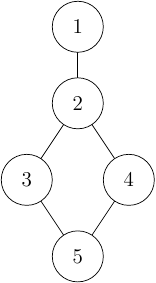
This implementation is very generic and can be used not only for rescuing our goat. For example think about looking for a path from 1 to 5 in the graph below.

Save the Goat (finally)

Let’s mix all together and save the goat before it starves or get eaten by the bad wolf.

start([a,a,a,a]).
goal([b,b,b,b]).

transition0([G,C,W,F1],[G,C,W,F2]).
transition0([F1,C,W,F1],[F2,C,W,F2]).
transition0([G,F1,W,F1],[G,F2,W,F2]).
transition0([G,C,F1,F1],[G,C,F2,F2]).

transition(X,Y) :- (transition0(X,Y);transition0(Y,X)), valid(X),valid(Y).

valid([F,_,_,F]).
valid([G,C,W,_]) :- G \== C, G \==W.

% Iterative Depth-Search Algorithm
ids_core(Node, Path, Goal, DepthLimit, ReturnPath) :-
    Node == Goal,reverse(Path,ReturnPath);
    transition0(Node,Neighbour),not(member(Neighbour,Path)),
    ids_core(Neighbour,[Node|Path],Goal,DepthLimit-1,ReturnPath).

ids_loop(Start,Goal,DepthLimit,ReturnPath) :-
    ids_core(Start,[Start],Goal,DepthLimit,ReturnPath);
    ids_loop(Start,Goal,DepthLimit+1,ReturnPath).

ids_start(Start,Goal,ReturnPath) :- ids_loop(Start,Goal,ReturnPath,1).

save_the_goat() :-
    start(S),
    goal(G),
    ids_start(S,G,R),
    write(R).